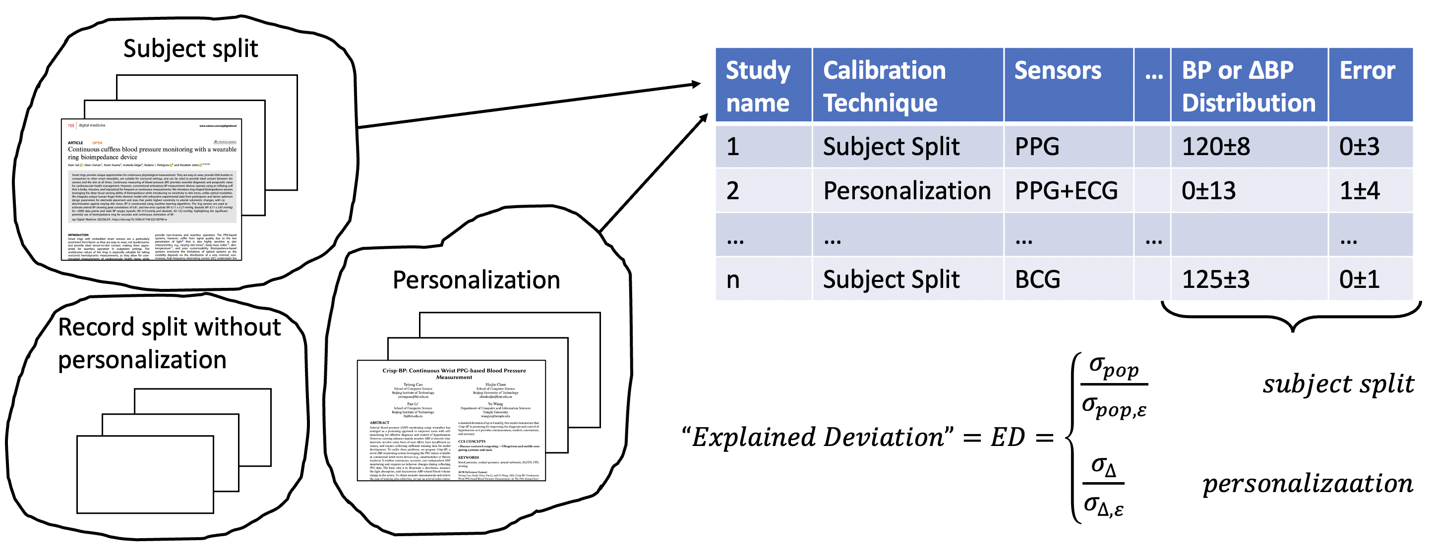
There is large heterogeneity in datasets, devices, and algorithms used in each study. Here, we provide an analysis that accounts for heterogeneity in dataset distributions and calibration techniques. We propose to do the following group studies by calibration technique, extract pertinent parameters, and compute a measure coined “Explained Deviation”.

Calibration Technique

We identified that there are three commonly used calibration methodologies: (a) subject split, (b) personalization, and (c) record split without personalization. Subject split involves using different subjects for the training and testing sets. A representative example is if 100 subjects are in the dataset, 50 subjects are used for training and the other 50 subjects for testing. Personalization allows subject data (a record) in training and testing sets but maintains causality in the data – training data only consists of data acquired before test data points. In other words, the training data is selected as the first portion of the record, and the testing data is selected as the latter portion, often with a clear, well-defined gap between training and test data. The training and testing data certainly do not overlap. For example, if a record for a single subject is one month long, data from the first day is used for training, and the rest is used for testing. This is used when the model’s generalization ability across the population of interest is unsatisfactory, so an individual-level model is fitted and recalibrated at arbitrary intervals due to physiological changes that may render the model inaccurate. Finally, some studies do not fall into these two categories, involving overlapping or non-causally split data in the training and testing set from the same subjects, thereby introducing data leakage. Examples are randomly sampled segments from a subject in training and test sets and fitting a model to all data to find correlations. We call this practice as record split without personalization. This type of calibration is not realizable in real-world practice because it violates causal constraints. Therefore, these studies were excluded from our analysis.
Metadata Statistics
To understand the distribution of extracted parameters for the studies included in our Systematic Review, we create interactive visualizations of of the different study parameter distributions. See Key for a description of extracted parameters.
Distribution of Sensors and Systems: ECG and PPG+ECG are the most used Sensors and Systems
<!DOCTYPE html>
Distribution of Algorithm Classes: Classical ML and Deep Learning are the most used algorithm classes.
<!DOCTYPE html>
Distribution of Datasets: Most datasets are private/internal. MIMIC is the most used publicly available dataset.
<!DOCTYPE html>
Distribution of Test Subject Characteristics: Most datasets only include either healthy or diseased subjects.
<!DOCTYPE html>
Distribution of Study Characteristics (observational or interventional): Most datasets are observational. Personalization studies are split between observational and interventional.
<!DOCTYPE html>
Distribution of Number of Test Subjects: Most datasets contain less than 300 testing subjects. Personalization studies tend to have lower number of testing subjects than subject split studies.
<!DOCTYPE html>
Distribution of Dataset SBP and DBP: Subject split studies tend to have larger BP STD compared to personalization change in BP STD. Relative magnitude of (change in) BP distribution is less for DBP.
<!DOCTYPE html>
<!DOCTYPE html>
Distribution of Study Power: Personalization studies tend to be less powered for <5±8mmHg on average.
<!DOCTYPE html>
Importance of accounting for BP Distribution in evaluation: BP Distribution is a confounding factor in BP Error
To determine whether the BP distribution affects the error we plot the standard deviation of the errors against the standard deviation of the BP distributions.
<!DOCTYPE html>
We find a significant relationship for both SBP and DBP. Studies with small distributions tend to have lower errors. Therefore, we must take BP distribution into account in analysis.
How time between calibration and test varies with error
To determine whether the accuracy of the personalization changes over time, we regress the error on the time between calibration and test (∆t). We plot time on the log (base-10) seconds scale
<!DOCTYPE html>
We find a significant relationship for both SBP and DBP, indicating that, overall, device accuracies wane over time.
Appendix 1: Power Analysis
Compute \(p=1-\beta=\phi(ES \sqrt{\frac{n}{2}}-z_{1-\alpha/2}))\) where \(ES\) (effect size) is given by error bias/error standard deviation=\(\frac{5}{8}\), \(\alpha\) is the selected level of significance, \(\beta=1-P\), and \(\phi\) is the cumulative distribution function of a normal distribution